Machine Learning for Insurance Claims
Andy Merlino
2018/09/18

We are pleased to announce a new demo Shiny application that uses machine learning to predict annual payments on individual insurance claims for 10 years into the future.
This post describes the basics of the model behind the above Shiny app, and walks through the model fitting, prediction, and simulation ideas using a single claim as an example.
Background
Insurance is the business of selling promises (insurance policies) to pay for potential future claims. After insurance policies are sold, it can be many years before a claim is reported to the insurer and many more years before all payments are made on the claim. Insurers carry a liability on their balance sheet to account for future payments on claims on previously sold policies. This liability is known as the Unpaid Claims Reserve, or just the Reserve. Since the Reserve is a liability for uncertain future payments, it’s exact value is not known and must be estimated. Insurers are very interested in estimating their Reserve as accurately as possible.
Traditionally insurers estimate their Reserve by grouping similar claims and exposures together and analyzing historical loss development patterns across the different groups. They apply the historical loss development patterns of the older groups (with adjustments) to the younger groups of claims and exposures to arrive at a Reserve estimate. This method does not accurately predict individual claim behavior, but, in aggregate, it can accurately estimate the expected value of the total Reserve.
Rather than using the traditional grouping methods, we predict payments on individual insurance claims using machine learning in R. Our goal is to model individual claim behavior as accurately as possible. We want our claim predictions to be indistinguishable from actual claims on an individual claim level, both in expected value and variance. If we can achieve this goal, we can come up with expected values and confidence levels for individual claims. We can aggregate the individual claims to determine the expected value and confidence levels for the total Reserve. There are many other insights we can gather from individual claim predictions, but let’s not get ahead of ourselves. Let’s start with an example.
Example - Predict Payments and Status for a Single Claim 1 Year into the Future
We will look at reported Workers’ Compensation claims. We will not predict losses on unreported claims (i.e. for our claim predictions, we already have 1 observation of the claim and we will predict future payments on this existing/reported claim). We will not predict future claims on policies that have not reported a claim to the insurer.
So our simplified model for 1 claims is:

We start with data for a single claim. Our goal is to predict the payments on our claim for 1 year into the future. We do this by feeding the claim to our payment model (which we will train later), and the model predicts the payments. Simple enough right? But we want to predict the status (“Open” or “Closed”) of the claim. We could do something like this:

Now we first predict the status, and then we predict the payments. We are getting closer to our goal now, but we also want to capture the variability in our prediction. We do this by adding a simulation after each model prediction:

The prediction returned by the above status model is the probability that the claim will be open at age 2 (e.g. our model might predict a 25% probability that our claim will be open at age 2. Since there are only 2 possible status states, “Open” or “Closed”, a 25% probability of being open implies a 75% probability the claim is closed at age 2). We use this probability to simulate open and closed observations of the claim. We then feed the observations (with simulated status) to our trained payment model. The payment model predicts an expected payment, and finally we simulate the variation in this expected payment based on the distribution of the payment model’s residuals.
If this sounds confusing, bear with me. I think a coded example will show it is actually pretty strait forward. Let’s get started:
Step 1: Load the data
Each claim has 10 variables. We have 3,296 claims in the training data and we pulled out 1 claim. We will make predictions for this 1 claim once we fit the models.
library(knitr)
library(kableExtra)
library(dplyr)

# This .RDS can be found at https://github.com/Tychobra/claims_ml_blog_post_data
data_training <- readRDS("../../static/data/model_fit_data.RDS")

test_claim_num <- "WC-114870"

# select one claim that we will make predictions for
test_claim <- data_training %>%
  filter(claim_num == test_claim_num)

# remove the one claim that we will predict from the training data
data_training <- data_training %>%
  filter(claim_num != test_claim_num)

knitr::kable(
  head(data_training)
) %>%
  kableExtra::kable_styling(bootstrap_options = "striped", font_size = 12) %>%
kableExtra::scroll_box(width = "100%") | claim_num | mem_num | cause_code | body_part_code | nature_code | class_code | status | paid_total | status_2 | paid_incre_2 |
|---|---|---|---|---|---|---|---|---|---|
| WC-163290 | Member A | Struck Or Injured | Skull | Amputation | 7720 | C | 6893.6947 | C | 451.3185 |
| WC-923705 | Member A | Struck Or Injured | Brain | Amputation | 9101 | C | 60247.1871 | C | 0.0000 |
| WC-808299 | Member A | Fall - On Same Level | Skull | Burn | 9101 | O | 34240.6365 | O | 2201.1637 |
| WC-536953 | Member A | Struck Or Injured | Skull | Contusion | 9015 | C | 599.8090 | C | 0.0000 |
| WC-146535 | Member A | Struck Or Injured | Skull | Contusion | 7720 | C | 265.5697 | C | 0.0000 |
| WC-523720 | Member A | Strain - Lifting | Skull | Concussion | 7720 | C | 85.8200 | C | 0.0000 |
The first column (“claim_num”) is the claim identifier and will not be used as a predictor variable in the model training. The 7 predictor variables (columns 2 through 8) represent the claim at age 1. The last 2 columns (“status_2” and “paid_incre_2”) are the variables we will predict. “status_2” is the claim’s status (“O” for Open and “C” for Closed) at age 2. “paid_incre_2” is the incremental payments made on the claim between age 1 and 2.
Step 2: Fit the Status Model
Our status model is a logistic regression, and we train it with the caret package. We use the step AIC method to perform feature selection.
library(caret)

# train the model
tr_control <- caret::trainControl(
  method = "none",
  classProbs = TRUE,
  summaryFunction = twoClassSummary
)

status_model_fit <- caret::train(
  status_2 ~ .,
  data = data_training[, !(names(data_training) %in% c("claim_num", "paid_incre_2"))],
  method = "glmStepAIC",
  preProcess = c("center", "scale"),
  trace = FALSE,
  trControl = tr_control
)


# create a summary to assess the model
smry <- summary(status_model_fit)[["coefficients"]]
smry_rownames <- rownames(smry)
out <- cbind(
  "Variable" = smry_rownames,
  as_data_frame(smry)
)

# display a table of the predictive variables used in the model
knitr::kable(
  out,
  digits = 3,
  row.names = FALSE
) %>%
  kableExtra::kable_styling(bootstrap_options = "striped", font_size = 12) %>%
kableExtra::scroll_box(width = "100%") | Variable | Estimate | Std. Error | z value | Pr(>|z|) |
|---|---|---|---|---|
| (Intercept) | -6.293 | 27.188 | -0.231 | 0.817 |
| cause_codeStrain | 0.174 | 0.057 | 3.036 | 0.002 |
| cause_codeStrike | 0.268 | 0.111 | 2.423 | 0.015 |
cause_codeStruck Or Injured
|
0.301 | 0.140 | 2.151 | 0.031 |
| body_part_codeSkull | -0.312 | 0.122 | -2.559 | 0.011 |
| nature_codeBurn | 0.266 | 0.123 | 2.168 | 0.030 |
| nature_codeContusion | -0.430 | 0.271 | -1.589 | 0.112 |
| nature_codeLaceration | 0.179 | 0.093 | 1.914 | 0.056 |
| nature_codeStrain | 0.156 | 0.066 | 2.365 | 0.018 |
| class_code8810 | 0.228 | 0.113 | 2.024 | 0.043 |
| class_code9102 | -2.706 | 144.101 | -0.019 | 0.985 |
| class_codeOther | 0.198 | 0.119 | 1.666 | 0.096 |
| statusO | 1.264 | 0.118 | 10.742 | 0.000 |
| paid_total | 0.184 | 0.048 | 3.862 | 0.000 |
The above table shows the variables that our step AIC method decided were predictive enough to keep around. The lower the p-value in the “Pr(>|z|)” column, the more statistically significant the variable. Not surprisingly “statusO” (the status at age 1) is highly predictive of the status at age 2.
Step 3: Fit the payment model
Next we use the xgboost R package along with caret to fit our payment model. We search through many possible tuning parameter values to find to the best values to tune the boosted tree. We perform cross validation to try to avoid over fitting the model.
library(xgboost)

xg_grid <- expand.grid(
  nrounds = 200, #the maximum number of iterations
  max_depth = c(2, 6),
  eta = c(0.1, 0.3), # shrinkage range (0, 1)
  gamma = c(0, 0.1, 0.2), # "pseudo-regularization hyperparameter" (complexity control)
  # range [0, inf]
  # higher gamma means higher rate of regularization.  default is 0
  # 20 would be an extremely high gamma and would not be recommended
  colsample_bytree = c(0.5, 0.75, 1), # range [0, 1]
  min_child_weight = 1,
  subsample = 1
)


payment_model_fit <- caret::train(
  paid_incre_2 ~ .,
  data = data_training[, !(names(test_claim) %in% c("claim_num"))],
  method = "xgbTree",
  tuneGrid = xg_grid,
  trControl = caret::trainControl(
    method = "repeatedcv",
    repeats = 1
  )
)
This trained model can predict payments on an individual claim like so:
test_claim_2 <- test_claim
test_claim_2$predicted_payment <- predict(
  payment_model_fit,
  newdata = test_claim_2[, !(names(test_claim_2) %in% c("claim_num", "paid_incre_2"))]
)

knitr::kable(
  test_claim_2
) %>%
  kableExtra::kable_styling(font_size = 12) %>%
kableExtra::scroll_box(width = "100%")| claim_num | mem_num | cause_code | body_part_code | nature_code | class_code | status | paid_total | status_2 | paid_incre_2 | predicted_payment |
|---|---|---|---|---|---|---|---|---|---|---|
| WC-114870 | Member A | Chemicals Burn | Skull | Burn | Other | O | 5517.135 | C | 1748.148 | 4103.079 |
The predicted payment (shown in the last column named “predicted_payment”) for our above claim was 4,103, and the actual payment between age 1 and 2 was 1,748. Our prediction was not extremely accurate, but it was at least within a reasonable range (or so it seems to me). Due to the inherent uncertainty in workers’ compensation claims, it is unlikely we will ever be able to predict each individual insurance claim with a high degree of accuracy. Our aim is to instead predict payments within a certain range with high accuracy. We use the following simulation technique to quantify this range.
Step 4: Use probility of being open to simulate the status
In our above prediction we used status at age 2 as a variable to predict the payment between age 1 and 2. Of course the actual status at age 2 will not yet be known when the claim is at age 1. Instead we can use our claim status model to simulate the status at age 2. We can then use this simulated status as a predictor variable.
# use status model to get the predicted probability that our test claim will be open
test_claim_3 <- test_claim

test_claim_3$prob_open <- predict(
  status_model_fit,
  newdata = test_claim_3,
  type = "prob"
)$O

# set the number of simulation to run
n_sims <- 200

set.seed(1235)
out <- data_frame(
  "sim_num" = 1:n_sims,
  "claim_num" = test_claim_3$claim_num,
  # run a binomial simulation to simulate the claim status `n_sims` times
  # this binomial simulation will return a 0 for close and 1 for open
  "status_sim" = rbinom(test_claim_3$prob_open, n = n_sims, size = 1)
)

# convert 0s and 1s to "C"s and "O"s
out <- out %>%
  mutate(status_sim = ifelse(status_sim == 0, "C", "O"))

kable(head(out)) %>%
kableExtra::kable_styling(font_size = 12)| sim_num | claim_num | status_sim |
|---|---|---|
| 1 | WC-114870 | C |
| 2 | WC-114870 | C |
| 3 | WC-114870 | C |
| 4 | WC-114870 | O |
| 5 | WC-114870 | C |
| 6 | WC-114870 | C |
The third column “status_sim” shows our simulated status. These are the values we pass the payment model (along with the 6 other predictor variables from age 1. We now have 200 observations of our single claim because we simulated the status 200 times. We can look at the number of times our claim was simulated to be open and closed like so:
table(out$status_sim)##
## C O
## 168 32Step 5: Predict a Payment for each of the simulated statuses
out <- left_join(out, test_claim, by = "claim_num") %>%
  mutate(status_2 = status_sim) %>%
  select(-status_sim)

out$paid_incre_fit <- predict(payment_model_fit, newdata = out)

knitr::kable(
  head(out)
) %>%
  kableExtra::kable_styling(font_size = 12) %>%
kableExtra::scroll_box(width = "100%")| sim_num | claim_num | mem_num | cause_code | body_part_code | nature_code | class_code | status | paid_total | status_2 | paid_incre_2 | paid_incre_fit |
|---|---|---|---|---|---|---|---|---|---|---|---|
| 1 | WC-114870 | Member A | Chemicals Burn | Skull | Burn | Other | O | 5517.135 | C | 1748.148 | 4103.079 |
| 2 | WC-114870 | Member A | Chemicals Burn | Skull | Burn | Other | O | 5517.135 | C | 1748.148 | 4103.079 |
| 3 | WC-114870 | Member A | Chemicals Burn | Skull | Burn | Other | O | 5517.135 | C | 1748.148 | 4103.079 |
| 4 | WC-114870 | Member A | Chemicals Burn | Skull | Burn | Other | O | 5517.135 | O | 1748.148 | 23163.445 |
| 5 | WC-114870 | Member A | Chemicals Burn | Skull | Burn | Other | O | 5517.135 | C | 1748.148 | 4103.079 |
| 6 | WC-114870 | Member A | Chemicals Burn | Skull | Burn | Other | O | 5517.135 | C | 1748.148 | 4103.079 |
The predicted payments are in the last column above. There predicted payment values differ depending on if the claim status was simulated to be open or closed. This gives us a little variability in our predicted payment, but it still does not capture the random variability of real world claims.
Step 6: Simulate Variability Around the Predicted Payment
Next we apply random variation to the predicted payment. For the sake of brevity here, we arbitrarily choose the negative binomial distribution, but in a real world analysis we would fit different distributions to the residuals to determine an appropriate model for the payment variability.
out$paid_incre_sim <- sapply(
  out$paid_incre_fit,
  function(x) {
    rnbinom(n = 1, size = x ^ (1 / 10), prob = 1 / (1 + x ^ (9 / 10)))
  }
)

knitr::kable(
  head(out)
) %>%
  kableExtra::kable_styling(font_size = 12) %>%
kableExtra::scroll_box(width = "100%")| sim_num | claim_num | mem_num | cause_code | body_part_code | nature_code | class_code | status | paid_total | status_2 | paid_incre_2 | paid_incre_fit | paid_incre_sim |
|---|---|---|---|---|---|---|---|---|---|---|---|---|
| 1 | WC-114870 | Member A | Chemicals Burn | Skull | Burn | Other | O | 5517.135 | C | 1748.148 | 4103.079 | 12706 |
| 2 | WC-114870 | Member A | Chemicals Burn | Skull | Burn | Other | O | 5517.135 | C | 1748.148 | 4103.079 | 4133 |
| 3 | WC-114870 | Member A | Chemicals Burn | Skull | Burn | Other | O | 5517.135 | C | 1748.148 | 4103.079 | 1120 |
| 4 | WC-114870 | Member A | Chemicals Burn | Skull | Burn | Other | O | 5517.135 | O | 1748.148 | 23163.445 | 15793 |
| 5 | WC-114870 | Member A | Chemicals Burn | Skull | Burn | Other | O | 5517.135 | C | 1748.148 | 4103.079 | 2015 |
| 6 | WC-114870 | Member A | Chemicals Burn | Skull | Burn | Other | O | 5517.135 | C | 1748.148 | 4103.079 | 1655 |
The payment we just simulated above (column “paid_incre_sim”) contains significantly more variability than our previously predicted payments. We can get a better sense of this variability with a histogram:
library(ggplot2)
library(scales)

payment_mean <- round(mean(out$paid_incre_sim), 0)
payment_mean_display <- format(payment_mean, big.mark = ",")

ggplot(out, aes(x = paid_incre_sim))+
  geom_histogram(color = "darkblue", fill = "white") +
  ylab("Number of Observations") +
  xlab("Predicted Payment") +
  ggtitle("Simulated Predicted Payments Between Age 1 and 2") +
  scale_x_continuous(labels = scales::comma) +
  geom_vline(
    xintercept = payment_mean,
    color = "#FF0000"
  ) +
  geom_text(
    aes(
      x = payment_mean,
      label = paste0("Simulation Mean = ", payment_mean_display),
      y = 10
    ),
    colour = "#FF0000",
    angle = 90,
    vjust = -0.7
  )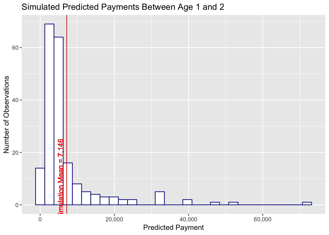
In the above plot we see our claim is predicted to have a payment anywhere from 0 to a little less than 80,000. The mean of the simulated prediction is 7,146 and the actual payments between age 1 and 2 now falls within our predicted range of possible payments. From a quick glance this distribution of possible claim payment values seems to be a reasonable representation of real world claim development.
There is still one additional easy alteration to make our simulated claim behave more like an actual claim. Actual claims have a fairly high probability of experiencing zero incremental payment over the upcoming year. We can test for the number of zero payment claims in our training data:
zero_paid <- data_training %>%
  filter(paid_incre_2 == 0)

# calculate the probability that a claim does not have any payement
prob_zero_paid <- nrow(zero_paid) / nrow(data_training)
69.9% of our claims have zero payment between ages 1 and 2. Our model currently does not make a clear distinction between claims with payment and claims with zero payment. A next step would be to fit another logistic regression to the probability of zero payment between age 1 and 2, and run a binomial simulation (just like our claim status simulation) to determine if the claim will have an incremental payment of zero or a positive incremental payment. We would also need to retrain our payment model using only the claims that had a positive payment between age 1 and 2 in the training set.
We will leave the zero payment model for you to try out on your own.
Why Run the Simulations
Often models are concerned with predicting the most likely outcome, the probability of an outcome, or the mean expected value. However, in insurance, we often are not as concerned with the mean, median, or mode outcome as we are with the largest loss we would expect with a high degree of confidence (e.g. We expect to pay no more than x at a 99% confidence level). Additionally, insurers are concerned with the loss payments they can expect to pay under various risk transfer alternatives (e.g. what is the expected loss if cumulative per claim payments are limited to 250,000 and aggregate losses per accident year over 1,000,000 are split 50%/50% between the insurer and a reinsurer). And what are the confidence levels for these risk transfer losses? With per claim predictions and simulations we can answer these questions for all risk transfer options at all confidence levels.
There is plenty of room for further improvement to this model, and there is a wide range of insights we could explore using individual claim simulations. Let me know your ideas in the comments.
comments powered by Disqus