Simulating Insurance Claims
Andy Merlino
2017/11/12

When I was fresh out of college, my boss asked me to run simulations in R. This was my first exposure to R. As someone with no programming experience, getting started was difficult. But with some Googling and a little perseverance, I worked through the initial frustration and am now a huge fan of the language. I hope this tutorial helps a beginning R user somewhere overcome one or two frustrations getting started.
This tutorial gives a basic introduction to simulations in R using an example from my first R project (simulating insurance claims). Random simulations are a nice beginner R project because they allow you to produce data and work with R’s data structures without ever even having to load data into R.
Step 1: Structure the Simulation to the Problem
Before we execute any R code, we need to describe the problem a little more fully. Let’s imagine that we own an insurance company and we are writing 100 identical insurance policies next year. We want to measure the losses we expect to pay on claims resulting from these policies. Our actuary tells us the probability of a single policy having a claim is 10%. Therefore we expect an average of 10 claims (10 = 100 * 0.1). We can use a discrete probability distribution to simulate the frequency (number of claims) based on this 10 claim average.
We then need to simulate a loss amount for each claim. We can use a continuous probability distribution for this simulation. Luckily our actuary already did her own historical claims analysis and informs us that claim severities follow a lognormal distribution with a log mean of 9 and a log standard deviation of 1.75 (In a real world simulation we could measure how well various distributions fit historical claims experience using several options available in R, but fitting distributions is beyond the scope of this tutorial).
Step 2: Run a Single Frequency/Severity Observation
We will refer to the combination of a frequency simulation and the accompanying severity simulations as an observation. Here we run one observation:
# set the seed so we can reproduce the simulation
set.seed(1234)

expected_freq <- 10

# generate a single frequency from the poisson distribution
freq <- rpois(n = 1, lambda = expected_freq)

# generate `freq` severities.  Each severity represents the ultimate value of 1 claim
# we will use the lognormal distribution here
sev <- rlnorm(n = freq, meanlog = 9, sdlog = 1.75)

# view the results
sev
## [1] 14046.732 15195.521  2256.730  8625.924  9874.455 98712.420
In the above example our frequency was 6, and our severities for each claim were 14,047, 15,196, 2,257, 8,626, 9,874, 98,712. By summing the severities of these 6 claims we arrive at the observation total of 148,712.
Step 3: Run Many Observations
Now that we know how to run a single observation we need to randomly generate a bunch of observations. By inspecting the results of many observations we can determine the confidence level of experiencing different loss amounts.
library(dplyr)
library(purrr)

# number of observations
n <- 1000
# generate many frequencies from the poisson distribution
freqs <- rpois(n = n, lambda = expected_freq)

# generate `freq` severities.  Each severity represents the ultimate value of 1 claim
obs <- purrr::map(freqs, function(freq) rlnorm(n = freq, meanlog = 9, sdlog = 1.75))

# tidy up the data
i <- 0
obs <- purrr::map(obs, function(sev) {
  i <<- i + 1
  data_frame(
    ob = i,
    sev = sev
  )
})
## Warning: `data_frame()` is deprecated, use `tibble()`.
## This warning is displayed once per session.

obs <- dplyr::bind_rows(obs)
head(obs, 10)
## # A tibble: 10 x 2
##       ob     sev
##    <dbl>   <dbl>
##  1     1  80356.
##  2     1  17897.
##  3     1 340101.
##  4     1  17256.
##  5     1   6110.
##  6     1   4648.
##  7     1   1335.
##  8     1   4504.
##  9     1  43360.
## 10     1   4187.
Step 4: Initial Inspection of Results
4.1: Plot the distribution of oberservations
library(ggplot2)

# aggregate claim severities by observation
obs_total <- obs %>%
  group_by(ob) %>%
  summarise(sev = sum(sev))

ggplot(obs_total, aes(sev)) +
  geom_histogram()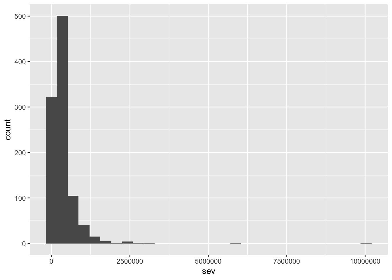
4.2: View some quantiles and summary info
quantile(obs_total$sev, probs = c(0.5, 0.75, 0.9, 0.95, 0.99))
##       50%       75%       90%       95%       99%
##  256185.5  435329.7  722109.2 1033543.0 1871843.3

summary(obs_total$sev)
##     Min.  1st Qu.   Median     Mean  3rd Qu.     Max.
##     2574   141666   256185   367565   435330 10030805
Step 5: Alter the simulation to specific needs
Assuming our initial inspection of the output in step 4 went as planned, we are ready to customize our simulation. We could adjust our simulation in a variety of different ways. Some common paths to take from here are:
5.1 Capping claims at individual claim limits
# cap claims at 250K
obs <- obs %>%
  dplyr::mutate(sev_250K = if_else(sev > 250000, 250000, sev))
5.2 Capping observations at an aggregate stop loss
# cap each observation at an aggregate stop loss
stop_loss <- 1000000

obs_agg <- obs %>%
  dplyr::group_by(ob) %>%
  dplyr::summarise(
    sev = sum(sev),
    sev_250K = sum(sev_250K)) %>%
  dplyr::mutate(
    sev_agg = if_else(sev > stop_loss, stop_loss, sev),
    sev_capped_agg = if_else(sev_250K > stop_loss, stop_loss, sev_250K)
  )

summary(obs_agg)
##        ob              sev              sev_250K          sev_agg
##  Min.   :   1.0   Min.   :    2574   Min.   :   2574   Min.   :   2574
##  1st Qu.: 250.8   1st Qu.:  141666   1st Qu.: 141666   1st Qu.: 141666
##  Median : 500.5   Median :  256185   Median : 256186   Median : 256186
##  Mean   : 500.5   Mean   :  367565   Mean   : 282172   Mean   : 328877
##  3rd Qu.: 750.2   3rd Qu.:  435330   3rd Qu.: 383357   3rd Qu.: 435330
##  Max.   :1000.0   Max.   :10030805   Max.   :1014342   Max.   :1000000
##  sev_capped_agg
##  Min.   :   2574
##  1st Qu.: 141666
##  Median : 256186
##  Mean   : 282158
##  3rd Qu.: 383357
##  Max.   :1000000
5.3: Simulate multiple types of claims
There is no reason the claims have to all be generated from the same distributions. We could simulate claims based on many different possible frequency and severity distributions. We could also add parameter risk to our frequency and severity selections. We could add deductibles, quota share reinsurance, and a variety of other alterations based our company’s needs.
Conclusion
Simulations are a fun way to get started in R, and with a little imagination, simulations allow you to answer highly complicated questions that would be impossible to solve directly from math equations and probability density functions.
comments powered by Disqus